The 📈Ups and 📉Downs of the San Francisco Construction Industry. Trends and History of the Construction

Category. Machine Learning
Tag. Analysis, Analytics, Big data, Building Permits, construction, mainpage, Open Data, San Francisco

This series of articles is devoted to the study of the construction activity of the main city of Silicon Valley — San Francisco. Charts and calculations were built with the help of Jupyter Notebook (Kaggle)

Data on more than a million building permits (records in two datasets) acquired from the San Francisco Construction Department allow us to analyze not only the construction activity in the city, but also critically examine the latest trends and development history of the construction industry over the past 40 years, from 1980 to 2019 (section “Annual Construction Activity in San Francisco”).

📈 The movement of activity in the construction industry in San Francisco almost completely coincides with the growth schedule for gold and bitcoin (section “The future of the San Francisco construction industry, pattern prediction”)

Open data provides an opportunity to explore the main factors that have influenced and will have an effect on the development of the construction industry in the city, dividing them into “external” (economic booms and crises) and “internal” (the effect of holidays and seasonal-annual cycles).

Content:

Open data and overview of initial parameters
Annual Construction Activity in San Francisco
Expectation and reality in drawing up the estimated cost
Construction activity depending on the season of the year
Total San Francisco Real Estate Investments
Areas of San Francisco that have received more investments over the past 40 years
Average estimated cost of application by city district
Monthly and Daily statistics on the total number of applications
The future of the San Francisco construction industry

1. Open data and overview of initial parameters.

San Francisco building permit data — taken from the open data portal — data.sfgov.org. The portal has several datasets on the topic of construction. Two such datasets store and update data on permits issued for the construction or repair of facilities in the city:

Building permits for the period 1980–2013 (850 thousand records)
Building permits for the period after 2013 (280 thousand records, data are downloaded and updated weekly)

These datasets contain information on the issued building permits with various characteristics of the facility for which the permit is issued. The total number of records (permits) received in the period 1980–2019 is 1,137,695 permits.

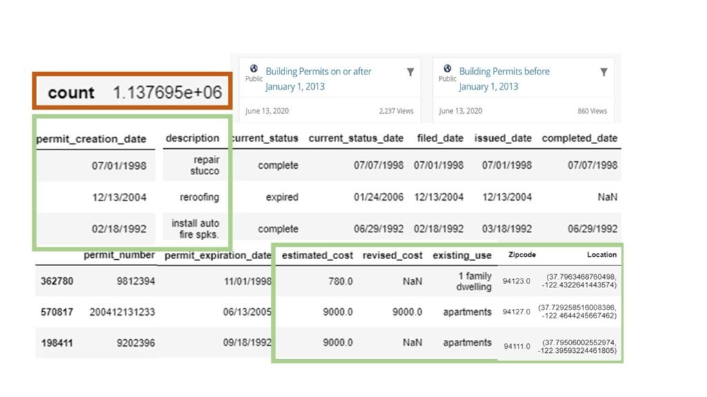
The main parameters from this dataset that were used for analysis:
permit_creation_date - date of creation of the permit (in fact, the day from which construction work begins)
description - description of the permit (two or three keywords describing the construction (work) object for which permission was created)
estimated_cost - estimated cost of construction work
revised_cost - cost of work after revaluation, increase or decrease of the initialvolume of the application
existing_use - type of housing (one-, two-family house, apartments, offices, etc.)
zipcode, location - zip code and coordinates of the object

Charts and calculations were built in the Jupyter Notebook (on the Kaggle.com platform).

2. Annual Construction Activity in San Francisco

In the graph below, the data on the estimated_cost and revised_cost parameters is presented as a distribution of the total cost of work by month (in billion US dollars).

data_cost_m = data_cost.groupby(pd.Grouper(freq='M')).sum()

📊 To reduce monthly “emissions”, monthly data is grouped by year. The graph of the amount of money invested over the years has received a more logical view and is amenable to analysis.

data_cost_y = data_cost.groupby(pd.Grouper(freq='Y')).sum()

By the annual movement of the sum of costs (all permits of the year) in urban facilities, it is seen that Economic factors from 1980 to 2019 have influenced the number and cost of construction projects or in other words, on San Francisco real estate investments.

The number of building permits (the number of construction works or the number of investments) over the past 40 years has been closely related to economic activity in the Silicone Valley.

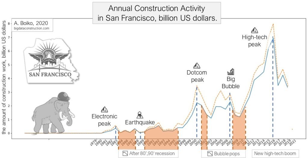
The first peak of construction activity was associated with the electronic hype of the mid-80s in the valley. The ensuing decline in electronics and banking in 1985 has led to the regional real estate market decline from which it has not yet recovered for nearly ten years.

🎢 Thereafter, the construction industry in San Francisco went through a parabolic growth of several thousand percent before the collapse of the Dotcom bubble and the technological boom of recent years. It happened two more times — in 1993–2000 and 2009–2016.

By removing the intermediate peaks and downturns and leaving the minimum and maximum values on each economic cycle, one can see how much large market fluctuations have plagued the industry over the past 40 years.

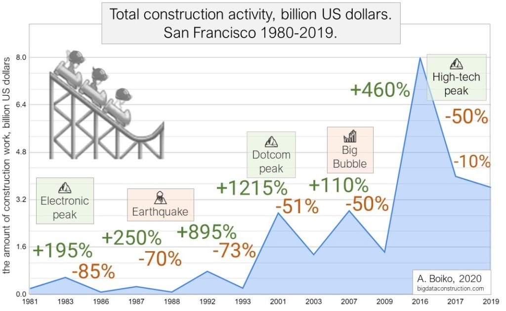
The largest investment increase in the field of construction occurred during the dot-com boom, when during the period from 1993 to 2001, $ 10 billion, or about $ 1 billion a year, were invested in repairs and construction. If you count in square meters (the cost of 1 m² in 1995 is $ 3,000) — this is approximately 350,000 m2 per year for 10 years, since 1993.

The growth of annual total investments for this period amounted to 1215%.

Companies that leased construction equipment during this period were like people who sold shovels during the gold rush (in the same region in the middle of the 19th century). Only instead of shovels — in the 2000s there were already cranes and concrete pumps for the newly formed construction companies who wanted to make money on the construction boom.

After each crisis that the construction industry has experienced over the years, over the next two post-crisis years, investments (the number of applications for permits) in construction fell each time by at least 50%.

The largest crises in the construction industry in San Francisco occurred in the 90s, were with a frequency of 5 years, the industry either fell (-85% between 1983–1986), then rose again (+ 895% between 1988–1992), remaining on the same level in annual terms — 1981, 1986, 1988, 1993.

🌊 After 1993, all subsequent downturns in the construction industry amounted to no more than 50%. But the approaching economic crisis (due to COVID-19) could create a record crisis in the construction industry in the period 2017–2021, the fall of which already for the period 2017–2019 amounts to more than 60%.

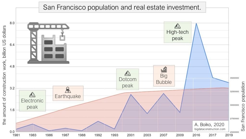
The population growth of San Francisco over the period 1980–1993 also showed almost exponential growth. The economic strength and innovative energy of Silicon Valley was the solid foundation upon which the hyperbole of the new economy, the American Renaissance and dotcoms was built. It was the epicenter of the new economy. But unlike the growth of real estate investments, after the peak of dotcoms, the population growth actually went to a plateau.

Since the 1950s and before the peak of the dotcoms in 2001, the annual population growth has been approximately about 1% per year. Later, after a housing bubble pop included a downturn in the economy, the influx of a new population has slowed down and since 2001 it has only been 0.2 % per year.

In 2019 (for the first time since 1950), the growth dynamics showed an outflow of the population (-0.21% or 7000 people) from the city of San Francisco.

3. Expectation and reality in drawing up the estimated cost

In the used datasets, data on the cost of permitting a building object is divided into:

initial estimated cost (estimated_cost)
cost of work after revaluation (revised_cost)

During the boom, the main purpose of revaluation is to increase the initial cost, when the investor (construction customer) shows a high interest in quality and volumes after the start of construction.

During the crisis — they tried not to exceed the estimated cost and the initial estimates , practically trying not to undergo changes (with the exception of the 1989 earthquake).

According to the graph of the revalued and estimated cost built on the difference (revised_cost — estimated_cost), we can observe that:

The amount of cost increase during the revaluation of the volume of construction work — directly depends on the cycles of the economic boom

data_spread = data_cost.assign(spread = (data_cost.revised_cost-data_cost.estimated_cost))

During periods of rapid economic growth customers (investors) spend their money generously enough, increasing their demands after the start of work.

The customer (investor), feeling his financial confidence, asks the construction contractor or an architect to expand the already issued building permit. This may be a decision to increase the initial length of the pool or increase the area of the house (after the start of work and the issuance of a building permit).

At the peak of dotcoms, such “additional” expenses reached the “extra” 1 billion per year.

If you look at this table as a percentage change, the peak increase in estimates (100% or 2 times the original estimated cost) came in the year before the earthquake in 1989 near the city. I suppose that after the earthquake (in 1989) the construction projects that were started in 1988 required more time and money to be implemented into it.

🌋 Conversely, a downward revision of the estimated cost (which happened only once during the period from 1980 to 2019) a few years before the earthquake is presumably due to the fact that some objects started in 1986–1987 were frozen or investments in these objects were cut back. According to the schedule, on average for each object begun in 1987, the estimated cost reduction was -20% of the original plan.

data_spread_percent = data_cost_y.assign(spread = ((data_cost_y.revised_cost-data_cost_y.estimated_cost)/data_cost_y.estimated_cost*100))

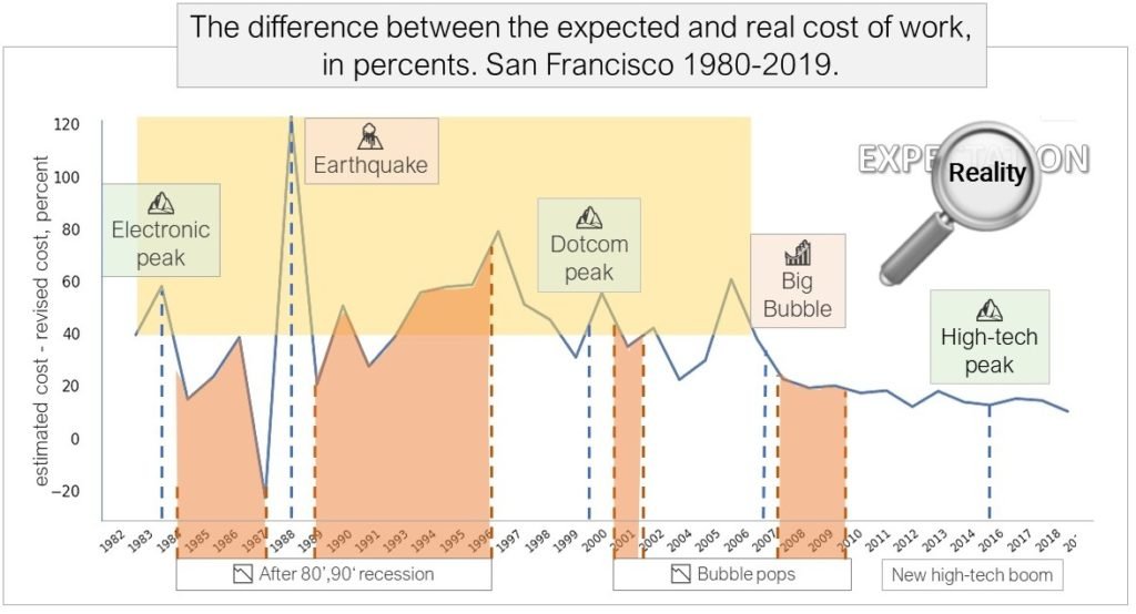
The increase in the initial estimated cost by more than 40% indicated or possibly was the result of an approaching bubble in the financial and subsequently the construction market.

What is the reason for the decrease in the spread (difference) between the estimated and revised sum after 2007?

Perhaps investors began to look at the numbers more carefully (the average investment over 20 years has increased from $ 100 thousand to $ 2 million dollars), or perhaps the construction department introduced new rules and restrictions to reduce possible manipulations and possible risks that arise during the crisis years in order to prevent and slow down the emerging bubbles in the real estate market.

4. Construction activity depending on the season of the year

Having grouped the data by calendar weeks in a year (54 weeks), you can observe the construction activity of the city of San Francisco, depending on seasonality and time of year.

🎅 By Christmas, all construction companies are trying to manage to get permission for new “large” objects (at the same time! The number! Permits in the same months are at the same level throughout the year). Investors, planning to get their property over the next year, conclude contracts in the winter months, counting on big discounts (since summer contracts, for the most part, are coming to an end by the end of the year and construction companies are interested in receiving new applications).

Before Christmas, the largest amounts are submitted in applications (an increase from an average of 1–1.5 billion per month. Up to 5 billion in December alone). At the same time, the total number of applications by month remains at the same level (see the section below: Statistics on the total number of applications by month and days)

After the winter holidays, the construction industry is actively (almost without an increase in the number of permits) planning and implementing “Christmas” orders, so that by the middle of the year (before the Independence Day) have time to free up resources before the beginning of immediately after the June holidays — a new wave of summer agreements.

data_month_year = data_month_year.assign(week_year = data_month_year.permit_creation_date.dt.week)data_month_year = data_month_year.groupby(['week_year'])['estimated_cost'].sum()

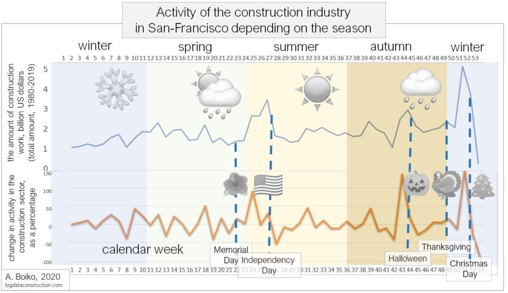
The same percentage data (orange line) also shows that the industry works “quietly” for a year, but before and after the holidays, permit activity increases to 150% between week 20–24 (before Independence Day), and decreases immediately after the holiday to -70%.

Before Halloween and Christmas, activity in the construction industry in San Francisco week 43–44 increases by 150% (from bottom to peak) and then decreases to zero during the holidays.

Therefore, the construction industry is in a six-month cycle, which is divided by the holidays “Independence Day of the USA” (week 20) and “Christmas” (week 52).

5. Total San Francisco Real Estate Investments

Based on the data on building permits in the city:

The total investment in construction projects in San Francisco from 1980 to 2019 is $ 91.5 billion.

sf_worth = data_location_lang_long.cost.sum()

The total market value of all residential real estate in San Francisco, estimated by property tax (is the estimated value of all real estate and all personal property owned by San Francisco) has reached $ 208 billion in 2016.

6. In which areas of San Francisco have invested more over the past 40 years

With the help of the Folium library, let’s see where these $ 91.5 billion by regions were invested. To do this, grouping the data by zip code (zipcode), imagine the value obtained using circles (Circle function from the Folium library).

import folium
from folium import Circle
from folium import Marker
from folium.features import DivIcon# map folium display
lat = data_location_lang_long.lat.mean()
long = data_location_lang_long.long.mean()
map1 = folium.Map(location = [lat, long], zoom_start = 12)for i in range(0,len(data_location_lang_long)):
    Circle(
        location = [data_location_lang_long.iloc[i]['lat'], data_location_lang_long.iloc[i]['long']],
        radius= [data_location_lang_long.iloc[i]['cost']/20000000],
        fill = True, fill_color='#cc0000',color='#cc0000').add_to(map1)
    Marker(
    [data_location_mean.iloc[i]['lat'], data_location_mean.iloc[i]['long']],
    icon=DivIcon(
        icon_size=(6000,3336),
        icon_anchor=(0,0),
        html='<div style="font-size: 14pt; text-shadow: 0 0 10px #fff, 0 0 10px #fff;; color: #000";"">%s</div>'
        %("$ "+ str((data_location_lang_long.iloc[i]['cost']/1000000000).round()) + ' mlrd.'))).add_to(map1)
map1

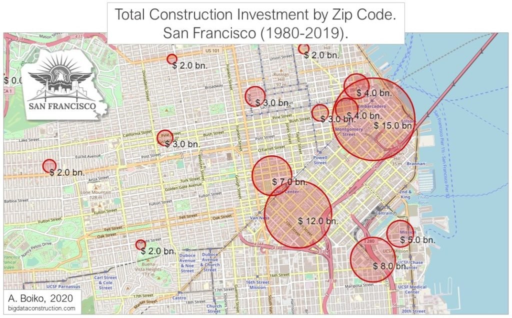
By looking at districts, it becomes clear that the majority of investments went to DownTown. Having simplified the grouping of all objects according to the distance to the city center and the time needed to get to the city center (of course, expensive houses are also being built on the coast), all permissions were divided into 4 groups: ‘Downtown’, ‘<0.5H Downtown’, ‘< 1H Downtown ‘,’ Outside SF ‘.

from geopy.distance import vincenty
def distance_calc (row):
    start = (row['lat'], row['long'])
    stop = (37.7945742, -122.3999445)    return vincenty(start, stop).meters/1000df_pr['distance'] = df_pr.apply (lambda row: distance_calc (row),axis=1)def downtown_proximity(dist):
    '''
    < 2 -> Near Downtown,  >= 2, <4 -> <0.5H Downtown
    >= 4, <6 -> <1H Downtown, >= 8 -> Outside SF
    '''
    if dist < 2:
        return 'Downtown'
    elif dist < 4:
        return  '<0.5H Downtown'
    elif dist < 6:
        return '<1H Downtown'
    elif dist >= 6:
        return 'Outside SF'
df_pr['downtown_proximity'] = df_pr.distance.apply(downtown_proximity)

91.5 billion that were invested in the city, almost 70 billion (75% of all investments) are invested in repairs and construction in the city center (green zone) and in the city area within a 2 km radius from the center (blue zone).

7. Average estimated cost of an application for construction by city district

All data, as in the case of the total amount of investments, was grouped by zip code. Only in this case with the average (.mean ()) estimated cost of the application by zip code.

data_location_mean = data_location.groupby(['zipcode'])['lat','long','estimated_cost'].mean()

In ordinary areas of the city (more than 2 km. From the city center) — the average estimated cost of an application for construction is $ 50 thousand.

The average estimated cost in the area of the city center is about three times higher ($ 150 thousand to $ 400 thousand) than in other areas ($ 30–50 thousand).

In addition to the cost of land, three factors determine the total cost of housing construction: labor, materials, and government fees. These three components are higher in California than in the rest of the country. California building codes are considered among the most comprehensive and stringent in the country (due to earthquakes and environmental regulations), often requiring more expensive materials and labor.

For example, the State requires builders to use higher quality building materials (windows, insulation, heating and cooling systems) to achieve high standards in energy efficiency.

From the general statistics on the average cost of an application for permission, two locations stand out favorably:

Treasure Island — is an artificial island in the San Francisco Bay. The average estimated cost of a building permit is $ 6.5 million.
Mission Bay — (lives 2926 people) The average estimated cost of a building permit is $ 1.5 million.

In fact, the highest average claim in these two areas is associated with the lowest number of applications for this zip code (145 and 3064 respectively, construction on the island is very limited), while for the rest of the postal codes for the period 1980–2019, approximately 1300 applications were received per year (total average of 30–50 thousand applications for the entire period).

By the parameter “number of permits” is noticeable a perfectly even distribution of the number of applications per zip code throughout the city.

8. Statistics on the total number of applications by month and day

General statistics on the number of applications by month and day from 1980 to 2019 shows that the “quietest” months for construction departments — are spring and winter months. At the same time, the amount of investments offered in the applications varies greatly, and it differs from month to month (see “Construction activity depending on the season of the year”). Among the days of the week on Monday, the department’s workload is approximately 20% less than the rest of the week.

data_month_count  = data_month.groupby(['permit_creation_date']).count()

While June and July practically do not differ in the number of applications, the difference in total estimated cost reaches 100% (4.3 billion in May and July and 8.2 billion in June).

data_month_sum  = data_month.groupby(['permit_creation_date']).sum()

9. The future of the San Francisco construction industry, pattern prediction.

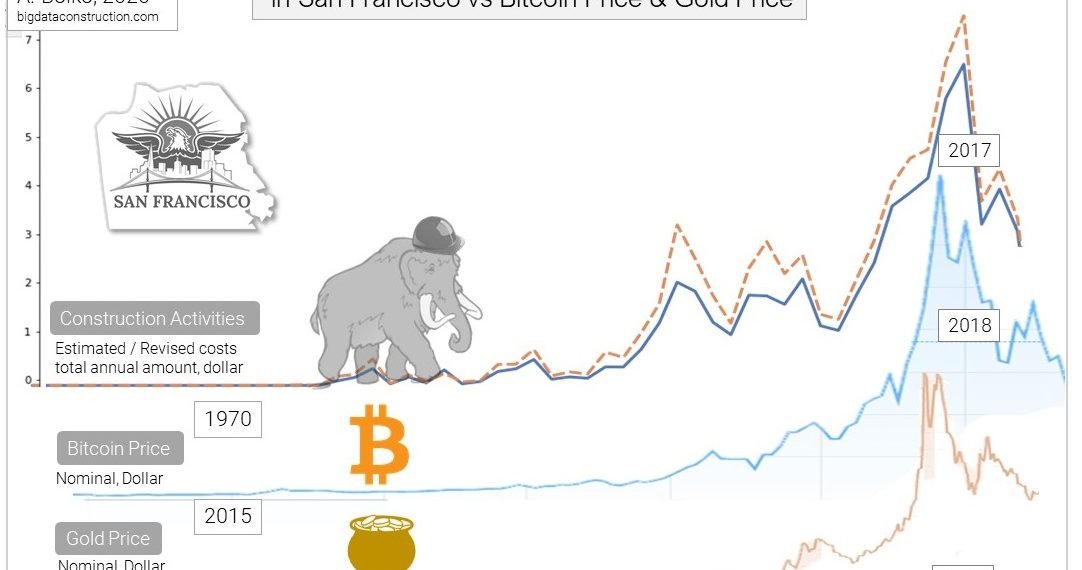
In conclusion, we compare the graph of construction activity in San Francisco with the graph of Bitcoin prices (2015–2018) and the graph of gold prices (1940–1980)

Pattern — in technical analysis is a stable repeated combinations of price, volume or indicator data. Pattern analysis is based on one of the axioms of technical analysis: “history repeats itself” — it is believed that repeated combinations of data lead to a similar result. Technical analysts have long used price patterns to examine current movements and forecast future market movements.

📈📉 Economic patterns have changed little from the ancient past to recent times. The main pattern that can be guessed on the annual activity chart is “Head and shoulders” — a trend reversal pattern. It is named because the graph looks like a human head (peak) and shoulders on the sides (smaller peaks). When the price breaks the line connecting the troughs, the pattern is considered complete, and the movement is likely to occur down.

The movement of activity in the construction industry in San Francisco almost completely coincides with the growth schedule for gold and bitcoin. The historical indicators of these three graphs of price and activity movement show significant similarities.

In the future, it is necessary to calculate the correlation coefficient with each of these two trends. Two random variables are called correlated if their correlation moment (or correlation coefficient) is nonzero, and are called uncorrelated quantities if their correlation moment is zero. If the obtained value is closer to 0 than to 1, then talking about a clear pattern does not make sense. This is a difficult mathematical problem, which senior comrades may possibly take on, who may be interested in this topic.

🔮 !Unscientific! we can look at the topic of further development of the San Francisco construction industry through the similarity of patterns. If the pattern matches further with the price of bitcoin, then according to this pessimistic option — coming out of the crisis in the construction industry in San Francisco will not be easy for the near post-crisis time.

With a more “optimistic” development option, a repeated exponential growth of the construction industry is possible if activity here goes according to the “gold price” scenario. In this option, in 20–30 years (maybe in 10), the construction sector expects a new surge in employment and development.

In the next part, I will take a closer look at individual sectors of construction (repair of roofs, kitchens, construction of stairs, bathrooms, and if you wish — for industries or other data; please leave me a comment) and compare inflation for individual types of work with Fixed Mortgage Rates & US Treasury Yield.

Link to Jupyter Notebook: San Francisco. Building sector 1980–2019.

Please, those who are registered on Kaggle — put a plus to this Notebook (Thank you!)(Notebooks will later add code comments and explanations)

🙋‍♂️ I will be glad to criticism, new proposals and opinion on regard of the tables. I will also be grateful for noting any spelling and logical errors. (Please indicate my mistakes made in English👏)

📈 More about various tools for working with big data visualization here: